Features

GPRSim.net это простая платформа для симуляции георадаров во временном пространстве. Программа частична основана на модели линии передач и позволяет симулировать до десяти слоев с частотами с 200 МГц до 2000 МГц. Её можно использовать для того чтобы попробовать разные условия зондирования в реальном мире. Это позволит понять как антенны с разными рабочими частотами могут повлиять на качество собираемых данных. Также поможно понять как сигнала может выглядеть в данных условиях. [Скачайте и попробуйте, программа бесплатна.]

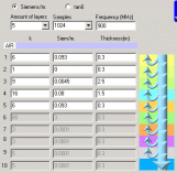Все слои характеризуются только тремя параметрами: относительная диэлектрическая проницаемость (эпсилон), электрическая проводимость (сигма) и физическая толщина слоя. Вместо электрической проводимости можно также ввести тангенс потери материала. Используемая модель предполагает что относительная магнитная проницаемость равна единице.

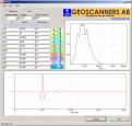
Результат симуляции представлен сразу как во временном так и в частотном пространствах, однако только график временного пространства можно отправить на печать. Можно сохранить разные условия симуляции в файлах типа CSV для последующей быстрой загрузки.

Временное а также частотное пространства имеют курсоры для более удобного толкования результатов симуляции. Таким образом можно рассчитать время прохождения через разные материалы. GPRSim.net показывает элементарные эффекты затухания сигнала для разных частот, а также возможные изменения фазы при прохождение через разные слои.

GPRSim.net может служить учебным пособием для изучения элементарных понятии о распространении электромагнитных волн через разные материалы. А так же поможет ответить на вопросы более общего рода как: как далеко можно проникнуть, какого наименьшего размера предмета можно обнаружить? Показывая разные сценарии зондирования с разными частотами можно довольно таки просто и наглядно показывать что ответ на эти вопросы далеко не простой и результаты зависят от многих факторов.

Наконец, эта программа предлагается абсолютно бесплатно для коммерческого или не коммерческого использования. Единственное ограничение это то, что вы не можете распространять её без заранее полученное письменное соглашение от нас.

Пожалуйста читаете инструкции по эксплуатации для того чтобы эффективно начать пользоваться GPRSim.net please read the user manual carefully. [руководство]

Не забудьте посмотреть учебник по георадарам [здесь] а также видеоучебник по использования программы [смотрите здесь].

В сотрудничестве с нашими партнерами из Matériel De Sondage s.a.r.l (MDS) во Франции мы смогли скомпилировать версию на французском языке. Сопровождающий файл помощи тоже был переведен на французский язык для удобства наших французко-говорящих пользователей. Французскую версию можно разгрузить [здесь].

[PAD File]

Отметка:

Изначально GPRSim.net называлась просто GPRSim что является сокращением для Ground Penetrating Radar Simulator. Из за того что уже существовала коммерческая программа под этим названием о которой мы не знали, то мы решили поменять название программы на GPRSim.net. Это было сделано в первую очередь для того чтобы избежать путаницы между этими двумя программами, но это не повлияло на работоспособность нашей программы. Мы благодарим всех кто разгрузил программу под старым названием и просим разгрузить новую версию.

G.P.R Basics using GPRSim.net

What is GPR?

GPR stands for Ground Penetrating Radar, also called Ground Probing Radar and as the name suggests it is a technique for probing the ground. Like any other radar it works by sending an electromagnetic wave into the ground and recording the returning signals. These returning signals contain information about the materials, or to be exact about the changes in materials or parameters of the ground at different depths.

It is appropriate to use GPR only if there are sharp differences in the properties of the materials being surveyed. If the differences of the materials are small or their changes are gradual then the returning signals are difficult to interpret and in many cases just impossible. [example]

GPR is well suited for geophysical applications, archeological surveys, and civil engineering applications and to locate hidden objects in the ground.

Are objects displayed like an X-ray picture?



A common misconception, mainly disseminated by Hollywood criminal television series and the like, is that the picture in the GPR control unit display presents objects as in an X-ray picture. Well, that’s not the case, the main working tool for GPR operators is the B-Scan which is nothing else than a collection of radar traces one after another in a 2D plot. (Picture on the right showing a B-Scan display of a survey)

If the picture is so unclear, why use GPR anyway?



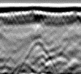
The advantages of using GPR are many; first of all it is a relatively inexpensive way of surveying large areas without destroying or corrupting anything. GPR provides an easy way of estimating depth to layers, ground waters, bedrock, caves and many other underground or under surface phenomena without the need for digging. Finding metallic pipes with a metal detector is an easy task; finding plastic pipes is impossible. GPR systems have no problem whatsoever to find metallic or non-metallic pipes, electrical cables hidden underground, concrete conduits etc.(Picture on the left showing a hyperbola in the B-Scan, which is typical for pipes)

Can one find a coin three meters under the ground?

No, that situation is unlikely to happen. The size and depth of the objects that can be detected are depending on the frequency and strength of the electromagnetic waves radiated into the ground by GPR transmitters with their antennas. They are also “illuminated” in a cone shape, the further into the material they travel the wider the area they cover, but the weaker they become. In order to see smaller objects the GPR antenna operating frequency most be raised, and in order to see deeper objects the operating frequency most be lowered. [example]

Does it always work?

No, as explained before GPR surveys are possible only if the properties of the materials under survey differ significantly. Further more, if the conductivity of the soil or the material under survey is very high then the penetration of the electromagnetic waves into the media is very limited if any at all. Soils with high content of minerals or clay are not good candidates for GPR surveys. [example]

Let’s try some examples and see how GPR works!

Before we go any further I’d like to remind a couple of things.

First, the simulation files are saved as CSV files with a special format. Every section has a linked CSV file so you don’t have to type in all the parameters, download the archive containing all the simulation files to some location in your hard disk and unzipped them to some location in your computer where you can find them later on.

Second, after the simulation is done it is possible to analyze the data in the time domain plot or in the frequency domain plot by moving the cursor of your mouse over the plot area. If some information should be gathered then press the left button on your mouse and see the measurement in the lower left corner of the application window.

Contrast of materials

If the properties of the materials we are trying to survey are not distinct enough then it becomes hard to detect them. We can use the concept of reflection coefficient to understand better the idea behind the materials contrast.

The reflection coefficient ρ (rho) is the ratio of the difference of the square roots of the relative dielectric constant of the two interface materials to the sum of the square roots of the dielectric constant of the two materials.



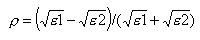
ε1 - relative dielectric constant of the material number one
ε2 - relative dielectric constant of the material number two
One thing about this equation, the material number one is the overlying material and the material number two is the underlying material.

The reflection coefficient can take positive or negative values, but for the purpose of this tutorial we are going to be concerned only with the absolute value of it not the sign. Then, it is correct to say that the reflection coefficient takes values ranging from zero to one. The closer the reflection coefficient gets to one the better for ground penetrating radar surveys.

Let’s take a look at what the radar trace would look like when the contrast of the materials is different or close to one another.

Example No. 1

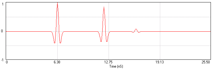
1. Open the simulation file sim1.csv. [download sim_files.zip] The simulation was set for running at 1GHz we will stick to this frequency since the materials contrast is what we want to see in this example. The contrast between the first and the second layer is good; the reflection coefficient is around 0.3. On the other hand the contrast between the second and the third layer is not that good and the reflection coefficient is roughly ten times less or 0.03. From this, one would imagine that the mid peak corresponding to the interface between the first and second layers will be strong while the last one corresponding to the interface between the second and the third layers will be weak.

2. From the view menu select 1:4 in order to see better what’s going o n, and press the
simulate button. A picture like this should appear.

Well, it seems that we got it right. The second peak is several times stronger than the last one, exactly as we expected it to be.

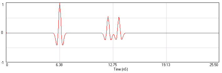
3. Try now to enter a new relative dielectric constant for the third layer, say 8.9 instead of 8 and press the simulate button again. What happened? The last peak almost disappeared, that is because the relative dielectric constant between the second and the third layer are so close that there’s almost no reflection at all.

Try out changing the relative dielectric constant of the different layers and running the simulation. An interesting value would be 18 for the last layer without changing the others. There’s a surprise there, see and try to find out when it happens and if interested enough, why it happens?

An interesting paper regarding this amplitude and phase changes in the presence of strong contrast between materials can be found here.

Resolution and penetration

The resolution and penetration that can be achieved with GPR are depending on many factors. Here, we will try to give an idea of the most important ones without entering in very deep detail, after all GPRSim.net is a very basic simulator good enough for simplified concepts only.

GPR resolution:

The concept of GPR resolution in its simplest form is nothing else than the smallest object the radar is capable to detect at a specific antenna operating frequency.

Let’s try out to detect the same object (layer in our software) with two different operating frequencies.

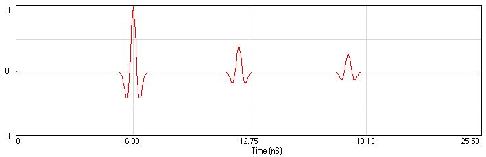
Example No. 2

1. Open the simulation file sim2.csv. [download sim_files.zip] The simulation was set for running at 1GHz from the start. Three layers have been defined, the top layer with a dielectric constant of 3 and a half meter thick. The second layer with a dielectric constant of 6 and very thin, only 8 cm thick and finally the last layer which is considered to be of infinite thickness. The conductivity of all layers was set equal and very low to avoid attenuation effects.

2. From the view menu select 1:4 in order to see better what’s going on.

3. Press the simulate button and a trace like this should appear.

The reflection from the interface between the top thick layer and the second thin one is clearly visible, that’s the peak in between the large one (surface) and the other small peak. It is possible to find without any problems the reflection from the interface between the thin layer and the last layer.

4. Now type in the frequency box 200. That’s the operating frequency for the new simulation.

5. Press the simulate button and see what happened.

All of the sudden the two small peaks disappeared and only a wide one appeared instead. It is impossible to say anything about this leave alone to detect the thickness of the first or second layer. Try out different frequencies and see what happens when the frequency goes up and down.

The previous example shows that what was clearly visible with an antenna operating at 1GHz is not recognizable with an antenna operating at 200MHz.

Now, does it mean higher frequency is always better? Let’s consider the next example.

Example No. 3

1. Open the simulation file sim3.csv. [download sim_files.zip] The simulation was set almost exactly in the same way as the example before just we added a bit of conductivity in order to make our point more clear to understand and made the mid layer somewhat thicker so the resolution was not an issue here.

2. From the view menu select 1:1 since this is a deeper survey simulation and we need as much range as possible.

3. Press the simulate button and a trace like this should appear.

Well, there’s nothing here except the surface reflection! What happened to the two meters layer? The 1GHz operating frequency antenna is very good at resolving thin layers near the surface as we saw from the previous example, but it appears to be useless when the second and third layers were some what deeper.

4. Now type in the frequency box 200. That’s the operating frequency for the new simulation.

5. Press the simulate button and see what happened. The two peaks indicating the two deep interfaces appeared and are clearly recognizable without trouble at all. What happened here is that the antenna with the operating frequency of 200 MHz reached deeper into the material, although at the expenses of resolution.

Try out reducing the thickness of the second layer while maintaining the same operating frequency and see what happens. An interesting value could be 10 cm, go ahead and see.

From example number three it was clear that higher frequency is not always better. The operating frequency of the antenna and GPR transmitter must be chosen according to the depth and the sizes of the objects we are trying to detect.

Attenuation

In the previous example we changed one parameter in order to make our point clear, that was the conductivity of the layers. How does it affect the GPR survey? The higher the conductivity of the materials we are trying to survey the higher the attenuation of the electromagnetic waves penetrating the media and therefore the less we can “see” into the ground. Highly electrical conductive media are salt water, and some types of clay particularly if they are wet. Agricultural soils containing soluble fertilizer like nitrogen or potassium can be highly conductive as well.

Let’s try out an example showing just that.

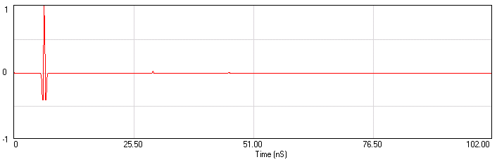
Example No. 4

1. Open the simulation file sim4.csv. [download sim_files.zip] The simulation was set to have three layers with the same conductivity and the dielectric constants were chosen so the peaks are spaced evenly from one another.

2. From the view menu select 1:4, which will allow us to see better what’s going to happen.

3. Press the simulate button and a trace like this should appear.

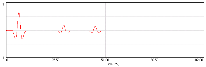
4. Now type in the conductivity box for the second layer 0.15, which is 150 milli Siemens/m. We have increased the conductivity ten times for the second layer.

5. Press the simulate button and see what happened. The third peak is now barely visible despite the fact that the contrast between the second layer and the third one hasn’t changed at all. So, what happened? The conductivity of the second layer became so high that almost all the energy was dissipated in it and there was almost nothing left to overcome the thickness of the last layer and be reflected back.

By changing the conductivity values it is possible to see how different media are more or less transparent to electromagnetic waves.

Try out changing the values of the conductivity and see how it will affect the GPR trace. By increasing the conductivity of the first layer the second and third become weaker. Try with more than three layers.

Depth to target

Velocity: The velocity of electromagnetic wave propagation through a physical media for most practical purposes can be defined as the ratio between the speed of light in vacuum and the square root of the relative dielectric constant of the media.

If the velocity of propagation through a media is known and the travel time through the media can be obtained then it is simple arithmetic to calculate the thickness of the media. This is strictly true only if the media is homogeneous and isotropic in space. Let’s try out an example to see how it works:

Example No. 5

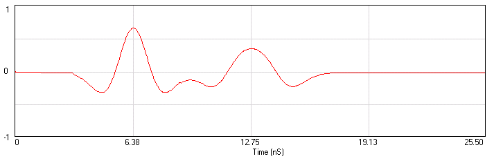
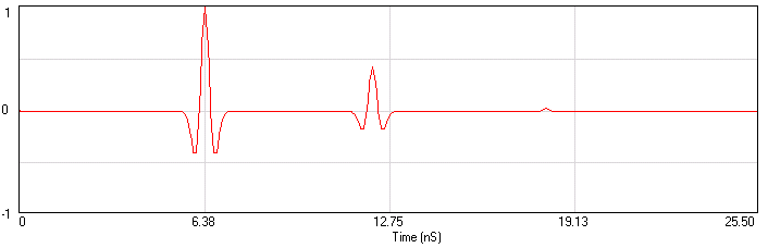
1. Open the simulation file sim5.csv [download sim_files.zip] as you can see there are only two layers in this simulation the first layer and the bottom one which is considered to be infinite.

2. From the view menu select 1:4 in order to get a clear view of the surface reflection and the one at the interface between the first and the second layer.

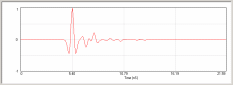
3. Press the simulate button and a trace like this should appear. The first wiggle is the reflection at the surface and the second is the reflection at the interface between the first and the second layers.

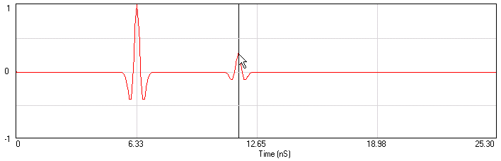
4. Put the cursor over the o-scope area and place the pointer over the highest positive peak and press the left button on your mouse in the left lower corner the time appears showing 6.33 nS. Now, put the cursor over the next highest positive peak and do the same as before. The time we got for this reflection is 11.7 nS.

5. The time difference between the first peak and the second one is 11.7nS - 6.33nS or 5.37nS. This is the time it takes for the electromagnetic wave to travel from the surface to the second layer and back.

6. The thickness of the layer can be calculated as:


D - Depth to the target or thickness of the layer
c - Speed of light in vacuum
t - Two way travel time
ε - Relative dielectric constant of the media

Putting the values in the equation gives us 0.2 meters thick layer and that’s exactly what we input in the layer thickness box.

In the real survey conditions the relative dielectric constant of the layer most be obtained first, by means of direct measurement or simply by estimation. The more homogeneous the media is and the more exact values for the relative dielectric constant, the more precise the depth measurements results.

Try out different simulations in order to get an idea of the needed range to observe feature underground.

The concepts explained above are the very basics of ground penetrating radar technology. By no means is this tutorial complete and/or exhaustive and many important concepts were left out, partly because it was not the purpose of this tutorial to be a survey design guide or anything like it and partly because features like scattering, focusing, ground coupling, near field effects and many more cannot be simulated in GPRSim.net.

Download this tutorial as a pdf file.